Which Kempner Partition Should Your Job Run On?

Which Kempner Partition Should Your Job Run On?#

A100 vs H100 vs H200 vs RTX6000, with benchmarks.

Author(s): Max Shad (Homepage) · Yasin Mazloumi (Homepage)

The Kempner AI cluster gives you a choice of GPU: A100, H100, H200, or RTX PRO 6000 (Blackwell). You can run jobs on all four base partitions, so the practical question is not whether you can get a GPU, but which one finishes your work fastest and with the least time spent waiting in the queue.

This post puts numbers behind that choice. We ran the same single-GPU benchmark on one GPU of each type and measured raw compute, memory bandwidth, and the throughput of a small transformer training step. The GPU Types and Use Cases page covers the full specifications and capabilities; here we focus on measured performance and a decision guide.

The four base partitions#

Each GPU type has its own SLURM partition. The RTX6000 nodes carry twice as many GPUs per node as the others.

GPU	Architecture	Partition	GPUs per node	Memory
A100	Ampere	`kempner`	4	40 GB HBM2
H100	Hopper	`kempner_h100`	4	80 GB HBM3
H200	Hopper	`kempner_h200`	4	141 GB HBM3e
RTX6000	Blackwell	`kempner_rtx`	8	96 GB GDDR7

How we measured#

We ran one identical PyTorch script on a single GPU of each type, under the same software stack (PyTorch 2.8, CUDA 12.8). It reports three things:

Compute: achieved throughput of a large square matrix multiply (16384 x 16384), timed with CUDA events, across precisions: TF32, FP16, BF16, and FP8. FP8 uses a scaled matrix multiply and runs only on the GPUs that support it. FP4 is Blackwell-only; we measured it separately on the RTX6000 with torchao and torch.compile (see Precision and special features).
Memory bandwidth: effective bandwidth of a 4 GiB device-to-device copy (reads plus writes).
Training throughput: a GPT-style transformer (16 layers, hidden size 2048, 16 heads, sequence length 1024, batch size 12, about 0.94 billion parameters) trained in bfloat16 with scaled dot-product attention and a fused AdamW step, reported as tokens per second. The model is sized to fit the 40 GB A100 so the same configuration runs on every GPU.

The large matrix multiply is chosen to keep the Tensor Cores busy, so the compute numbers land close to what each GPU can sustain. We ran each benchmark on three independent GPU allocations and report the mean, with error bars for one standard deviation. These are single-GPU numbers with no multi-GPU or multi-node scaling. Matmul figures are achieved throughput, not vendor peak, and the training number is for this specific model; treat them as a realistic guide rather than a hard ceiling. The Reproduce it yourself section has the full script.

Benchmark results#

The A100 has the least compute and memory. The H100 and H200 lead on compute and match within run-to-run variation. The H200 pulls ahead on memory bandwidth and, with it, end-to-end training throughput. FP8 roughly doubles matrix multiply throughput on the GPUs that support it, and the RTX6000 sits in the middle. The matrix multiply figure and the bandwidth and training figure below break this down.

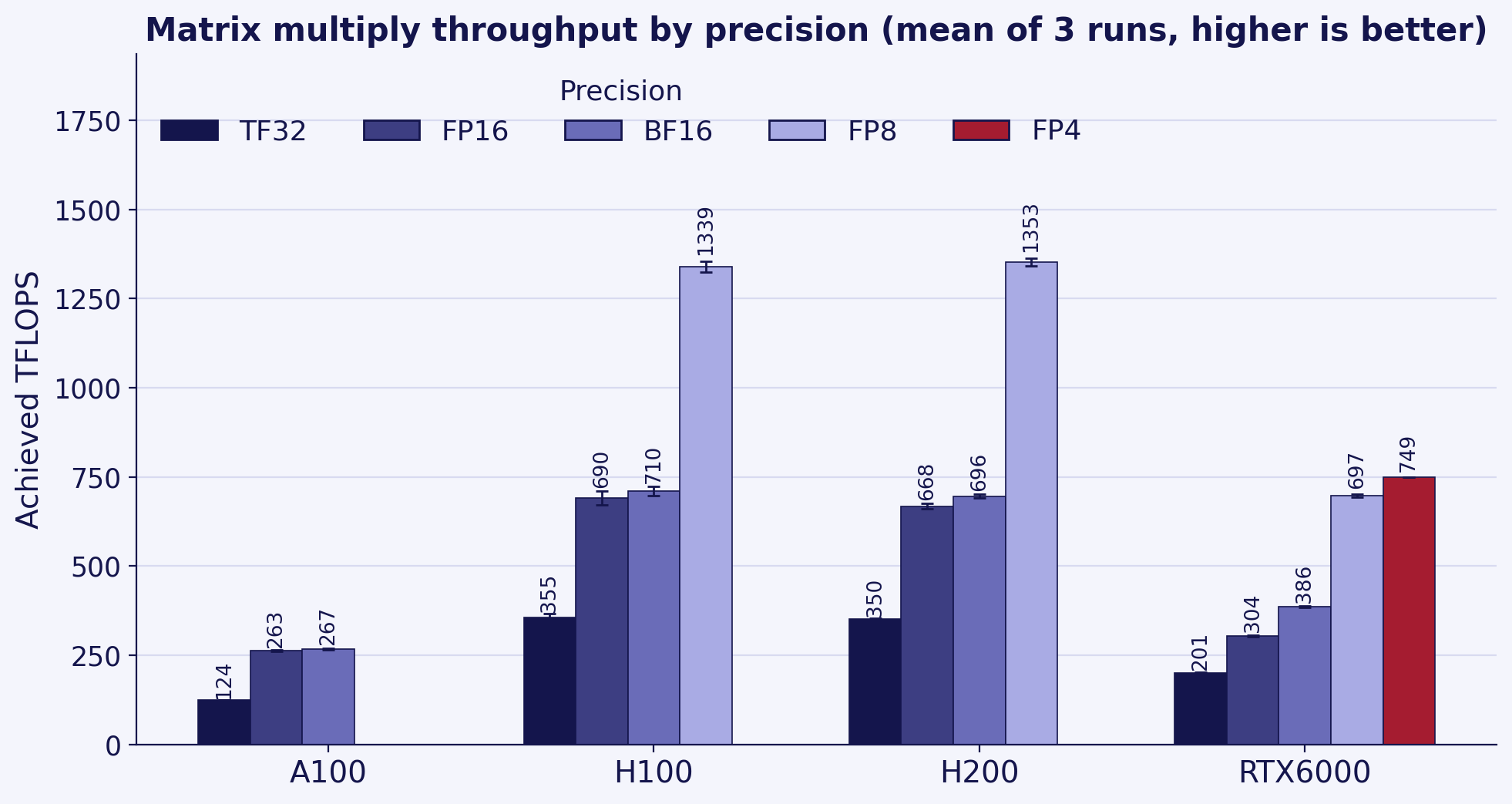
../_images/compute_tflops.png — Fig. 1 Achieved matrix multiply throughput (16384 x 16384) by precision. Each bar is the mean of three runs, and the error bars show one standard deviation. FP8 runs on the H100, H200, and RTX6000; FP4 (crimson) is unique to the RTX6000, and the A100 supports neither. The FP4 bar uses the torchao NVFP4 path with torch.compile, the fastest FP4 route available on this GPU.#

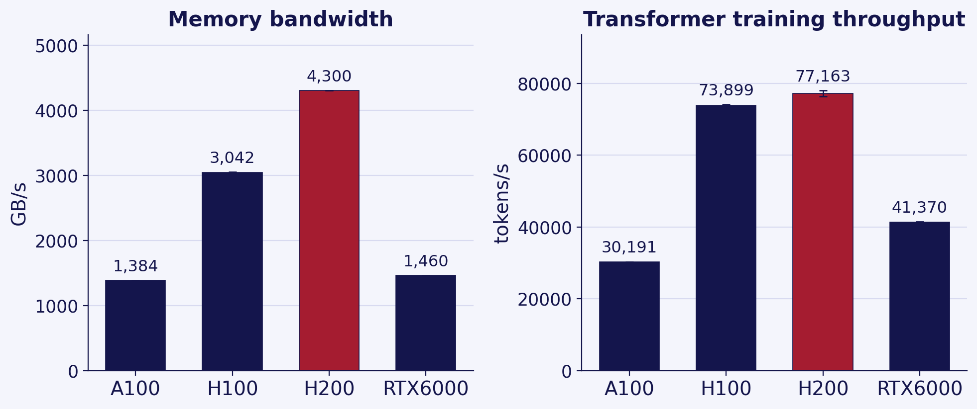
../_images/bandwidth_throughput.png — Fig. 2 Left: effective memory bandwidth from a 4 GiB device-to-device copy. Right: throughput of one bfloat16 training step of a 0.94 billion parameter transformer. Bars are the mean of three runs, with error bars for one standard deviation. The H200 (crimson) leads both, and end-to-end training tracks memory bandwidth as much as raw compute.#

The measured numbers:

GPU	TF32	FP16	BF16	FP8	FP4	Bandwidth (GB/s)	Training (tokens/s)
A100	124	263	267	n/a	n/a	1,384	30,191
H100	355	690	710	1,339	n/a	3,042	73,899
H200	350	668	696	1,353	n/a	4,300	77,163
RTX6000	201	304	386	697	749	1,460	41,370

Each value is the mean of three runs. The TF32 through FP8 columns are achieved matrix multiply throughput in TFLOPS. FP8 runs only on the H100, H200, and RTX6000. FP4 is unique to the RTX6000; its value uses the torchao NVFP4 path with torch.compile, the fastest FP4 route we found on this GPU, so it is not directly comparable to the raw-matmul columns.

A few things stand out:

Compute: the two Hopper GPUs match, as expected. They share the same compute architecture, and across three runs they agree within run-to-run variation: BF16 was 710 ± 14 TFLOPS on the H100 and 696 ± 5 on the H200, and on FP8 the H200 was a touch higher (1,353 against 1,339). At BF16 both land about 2.6 times the A100 and 1.8 times the RTX6000.
FP8 roughly doubles throughput where it is available. On the H100, H200, and RTX6000, FP8 matrix multiply ran about 1.8 to 1.9 times faster than BF16 (1,339 against 710 TFLOPS on the H100, for example). The A100 has no FP8.
FP4 works on the RTX6000, and it is early. FP4 is unique to the Blackwell RTX6000. Reaching its fast path took the torchao NVFP4 inference route with torch.compile, which hit about 749 TFLOPS, just above the same GPU’s FP8. A raw FP4 matmul was several times slower, which points to FP4 software for this GPU still maturing rather than a hardware limit.
Bandwidth: the H200 is in a class of its own. Its HBM3e delivers about 4,300 GB/s, roughly 40 percent more than the H100 and about three times the A100 and RTX6000. The RTX6000 GDDR7 memory lands near the A100, well below the Hopper HBM.
Training tracks bandwidth, not just compute. The H100 and H200 are close on compute, but the H200 trains this model a few percent faster, because the step is partly memory bound. Both Hopper GPUs are roughly 2.5 times the A100, and the RTX6000 trains it about 37 percent faster than the A100.
Memory capacity sets the ceiling. The A100 has 40 GB, the H100 80 GB, the H200 141 GB, and the RTX6000 96 GB. That ceiling, not speed, is often what decides whether a model and its batch fit at all.

These are single-GPU, achieved numbers for one specific workload, not vendor peak values and not multi-GPU scaling. Treat them as a realistic guide to relative performance rather than a guarantee for every job.

Precision and special features#

Beyond raw speed, the four GPUs differ in which numerical formats and hardware features they support. That often matters more than a throughput number, because it decides whether a technique is available to you at all.

FP16 and BF16 (all four GPUs). Both are 16-bit formats and the everyday choice for mixed-precision training and inference. On the Hopper GPUs FP16 and BF16 run at essentially the same speed, so BF16 is usually preferred for its wider dynamic range.
FP8 (H100, H200, RTX6000). The Hopper and Blackwell Tensor Cores add FP8, which roughly doubled matrix multiply throughput over BF16 in our runs (about 1.8 to 1.9 times). It is the format for the highest-throughput large-model training and inference. The A100 does not support it.
FP4 (RTX6000 only). The Blackwell RTX6000 adds FP4 for aggressive low-precision and quantization work. With torchao and torch.compile, FP4 reached about 749 TFLOPS, just above the RTX6000 FP8 rate. The fast path is still narrow: a plain FP4 matmul was several times slower, so FP4 is the format to watch for quantized inference as its software matures. See GPU Types and Use Cases.
RT Cores (RTX6000 only). The RTX6000 is the only GPU here with ray-tracing cores. They do not help matrix math, so they do not show up in the benchmark, but they accelerate rendering and the simulation behind robotics and reinforcement learning.

The compute figure above shows FP8 bars only on the H100, H200, and RTX6000, a direct picture of where that capability is available.

Which partition should you pick?#

The right partition depends on the workload. For large multi-GPU training that shards one model, the NVLink Hopper GPUs (H100 and H200) scale best, with the H200 adding the most memory and bandwidth. For single-GPU work, the RTX6000 is a strong general-purpose choice: with 96 GB, more than the H100, and solid throughput, it handles single-GPU training, fine-tuning, inference, and reinforcement-learning experiments, and it also carries FP4 and RT Cores. The Hopper GPUs pull ahead when you need the fastest single-GPU compute or multi-GPU scaling, and the A100 suits smaller or exploratory jobs that fit its 40 GB.

        flowchart TD
    A[Start: which partition?] --> B{Multi-GPU training that<br/>shards one model over NVLink?}
    B -->|Yes| C{Needs the most<br/>memory or bandwidth?}
    C -->|Yes| H200a["kempner_h200: H200, 141 GB"]
    C -->|No| H100a["kempner_h100: H100, 80 GB"]
    B -->|No| D{Want peak compute<br/>throughput?}
    D -->|Yes| E{Over 80 GB or<br/>bandwidth bound?}
    E -->|Yes| H200b["kempner_h200: H200, 141 GB"]
    E -->|No| H100b["kempner_h100: H100, 80 GB"]
    D -->|No| F{Small or exploratory job<br/>that fits in 40 GB?}
    F -->|Yes| A100["kempner: A100, 40 GB"]
    F -->|No| RTX["kempner_rtx: RTX6000, 96 GB"]

The table below maps common workloads to a recommended partition.

Workload	Recommended partition	Why
Largest models, long context, memory-bound inference	`kempner_h200`	Most memory (141 GB) and highest bandwidth
High-throughput large-model training with FP8	`kempner_h100` or `kempner_h200`	Hopper Tensor Cores and FP8
Single-GPU training, fine-tuning, inference, or RL	`kempner_rtx`	96 GB on one GPU with good throughput, no NVLink needed
Low-precision or quantization research (FP4)	`kempner_rtx`	Only GPU here with FP4
Rendering, robotics, reinforcement learning with simulation	`kempner_rtx`	RT Cores for ray tracing
Small to mid-size training and prototyping	`kempner` (A100)	Widely available, well understood
Sharding one model across many GPUs	`kempner_h100` or `kempner_h200`	NVLink scales better than the RTX6000 PCIe link

Practical notes: queue, caps, and how to request#

Requesting a partition. Submit to the matching partition, for example salloc -p kempner_h200 --account=<your_account> --gres=gpu:1, or the same -p flag in an sbatch script. See Job Submission Basics.
GPU caps. Usage across the four base partitions is capped per user and per account; see Cluster Usage Policies.
When a partition is busy. The kempner_requeue partition is not subject to the base-partition caps and is a good place to soak up spare capacity, as long as your job checkpoints, since higher-priority work can preempt it.

Reproduce it yourself#

All four runs used the same script on a single GPU, under PyTorch 2.8.0 with CUDA 12.8. Each job requested one GPU on the matching partition, for example:

sbatch -p kempner_h200 --account=<your_account> --gres=gpu:1 -c 16 --mem=64G \
       -t 0-00:20 --wrap "python gpu_bench.py --tag h200"

Swap the partition (kempner, kempner_h100, kempner_h200, kempner_rtx) to target each GPU type. The script times matrix multiplies with CUDA events across precisions, a 4 GiB device-to-device copy, and a transformer training step, and prints one JSON line of results.

FP4 on the RTX6000 was measured separately, since it needs a low-precision library: we installed torchao and timed an NVFP4 linear with dynamic activation quantization, compiled with torch.compile, which was the fastest FP4 path we found in this stack.

Full benchmark script (gpu_bench.py)

import argparse
import json
import torch

MATMUL_N = 16384
MATMUL_ITERS = 50
MATMUL_WARMUP = 10

# Transformer training config (fits the 40 GB A100 with margin).
CFG = dict(vocab=32000, d=2048, h=16, layers=16, seq=1024, batch=12, steps=30, warmup=8)


def time_cuda(fn, iters, warmup):
    for _ in range(warmup):
        fn()
    torch.cuda.synchronize()
    start = torch.cuda.Event(enable_timing=True)
    end = torch.cuda.Event(enable_timing=True)
    start.record()
    for _ in range(iters):
        fn()
    end.record()
    torch.cuda.synchronize()
    return start.elapsed_time(end) / iters / 1000.0  # seconds per iter


def matmul_tflops(dtype, n, iters, warmup):
    a = torch.randn(n, n, device="cuda", dtype=dtype)
    b = torch.randn(n, n, device="cuda", dtype=dtype)
    t = time_cuda(lambda: torch.matmul(a, b), iters, warmup)
    return (2.0 * n ** 3) / t / 1e12


def matmul_tflops_fp8(n, iters, warmup):
    a = torch.randn(n, n, device="cuda", dtype=torch.bfloat16).to(torch.float8_e4m3fn)
    b = torch.randn(n, n, device="cuda", dtype=torch.bfloat16).to(torch.float8_e4m3fn)
    b = b.t().contiguous().t()  # scaled_mm wants the second operand column-major
    scale = torch.tensor(1.0, device="cuda", dtype=torch.float32)

    def fn():
        torch._scaled_mm(a, b, scale_a=scale, scale_b=scale,
                         out_dtype=torch.bfloat16, use_fast_accum=True)

    t = time_cuda(fn, iters, warmup)
    return (2.0 * n ** 3) / t / 1e12


def bandwidth_gbps(nbytes, iters, warmup):
    n = nbytes // 4
    src = torch.empty(n, device="cuda", dtype=torch.float32).normal_()
    dst = torch.empty(n, device="cuda", dtype=torch.float32)
    t = time_cuda(lambda: dst.copy_(src), iters, warmup)
    return (2.0 * nbytes) / t / 1e9  # read + write


class Block(torch.nn.Module):
    def __init__(self, d, h):
        super().__init__()
        self.h = h
        self.ln1 = torch.nn.LayerNorm(d)
        self.ln2 = torch.nn.LayerNorm(d)
        self.qkv = torch.nn.Linear(d, 3 * d)
        self.proj = torch.nn.Linear(d, d)
        self.fc1 = torch.nn.Linear(d, 4 * d)
        self.fc2 = torch.nn.Linear(4 * d, d)

    def forward(self, x):
        b, t, d = x.shape
        qkv = self.qkv(self.ln1(x)).view(b, t, 3, self.h, d // self.h).permute(2, 0, 3, 1, 4)
        q, k, v = qkv[0], qkv[1], qkv[2]
        a = torch.nn.functional.scaled_dot_product_attention(q, k, v, is_causal=True)
        a = a.transpose(1, 2).contiguous().view(b, t, d)
        x = x + self.proj(a)
        x = x + self.fc2(torch.nn.functional.gelu(self.fc1(self.ln2(x))))
        return x


class GPT(torch.nn.Module):
    def __init__(self, vocab, d, h, layers, seq):
        super().__init__()
        self.tok = torch.nn.Embedding(vocab, d)
        self.pos = torch.nn.Embedding(seq, d)
        self.blocks = torch.nn.ModuleList([Block(d, h) for _ in range(layers)])
        self.lnf = torch.nn.LayerNorm(d)
        self.head = torch.nn.Linear(d, vocab, bias=False)

    def forward(self, idx):
        b, t = idx.shape
        x = self.tok(idx) + self.pos(torch.arange(t, device=idx.device))
        for blk in self.blocks:
            x = blk(x)
        return self.head(self.lnf(x))


def train_tokens_per_sec(cfg):
    model = GPT(cfg["vocab"], cfg["d"], cfg["h"], cfg["layers"], cfg["seq"]).cuda()
    try:
        opt = torch.optim.AdamW(model.parameters(), lr=1e-4, fused=True)
    except (RuntimeError, ValueError):
        opt = torch.optim.AdamW(model.parameters(), lr=1e-4)
    idx = torch.randint(0, cfg["vocab"], (cfg["batch"], cfg["seq"]), device="cuda")
    tgt = torch.randint(0, cfg["vocab"], (cfg["batch"], cfg["seq"]), device="cuda")

    def step():
        opt.zero_grad(set_to_none=True)
        with torch.autocast("cuda", dtype=torch.bfloat16):
            logits = model(idx)
            loss = torch.nn.functional.cross_entropy(
                logits.view(-1, cfg["vocab"]), tgt.view(-1))
        loss.backward()
        opt.step()

    t = time_cuda(step, cfg["steps"], cfg["warmup"])
    return (cfg["batch"] * cfg["seq"]) / t


def main():
    ap = argparse.ArgumentParser()
    ap.add_argument("--tag", default="gpu")
    args = ap.parse_args()

    torch.backends.cuda.matmul.allow_tf32 = True
    torch.backends.cudnn.allow_tf32 = True
    torch.backends.cudnn.benchmark = True

    res = {"tag": args.tag}
    props = torch.cuda.get_device_properties(0)
    res["gpu_name"] = props.name
    res["mem_gb"] = round(props.total_memory / 1e9, 1)

    def safe(key, fn):
        try:
            res[key] = round(fn(), 1)
        except Exception as ex:
            res[key] = None

    safe("tf32_tflops", lambda: matmul_tflops(torch.float32, MATMUL_N, MATMUL_ITERS, MATMUL_WARMUP))
    safe("fp16_tflops", lambda: matmul_tflops(torch.float16, MATMUL_N, MATMUL_ITERS, MATMUL_WARMUP))
    safe("bf16_tflops", lambda: matmul_tflops(torch.bfloat16, MATMUL_N, MATMUL_ITERS, MATMUL_WARMUP))
    safe("fp8_tflops", lambda: matmul_tflops_fp8(MATMUL_N, MATMUL_ITERS, MATMUL_WARMUP))
    safe("bandwidth_gbps", lambda: bandwidth_gbps(4 * 1024 ** 3, 50, 10))
    safe("train_tok_s", lambda: train_tokens_per_sec(CFG))

    print("RESULT_JSON " + json.dumps(res))


if __name__ == "__main__":
    main()

Summary#

You can run on all four base partitions, so pick by fit, not just by whatever is free at the moment.
For compute-bound training and inference, the H100 and H200 are effectively tied and well ahead of the A100 and RTX6000.
When a job is memory-bound, or needs the most memory or bandwidth, the H200 is the clear pick.
The RTX6000 is a strong general-purpose single-GPU option, with 96 GB and the only FP4 and RT Cores here. The A100 remains a fine choice for small or established work.
Check current queue depth and the per-user and per-account GPU caps before committing a large job, and use kempner_requeue to soak up spare capacity.