19.3. GPU Profiling#
This section explains how to profile GPUs to design a better performant code. GPU profiling helps to get some insights of GPUs behavior to identify and fix performance bottlenecks. The following steps are performed iteratively until achieving the desired performance:
Profile the code
Analyze the traces to identify the possible performance bottlenecks
Fix the bottlenecks and optimize the code.

Fig. 19.5 Profiling Loop to Optimize Code#
19.3.1. Profiling using Pytorch Profiler#
PyTorch profiler is a tool that facilitates collecting different performance metrics at runtime to better understand what happens behind the scene. For example, during training of a ML model, torch profiler can be used for understanding the most expensive model operators, their impact and studying device kernel activity. More particularly to answer the following questions:
How much GPU run time contributes to Computation, Communication or Memory related kernels.
How much these different categories overlap one another (non-blocking kernel calls or multiple parallel cuda streams can be used to provide overlapping).
What kernels are the most expensive ones within the above categories (breakdown).
Following shows how we can wrap the training loop to be performed in the context of the torch profiler using with statement.
from torch.profiler import profile, schedule, tensorboard_trace_handler

tracing_schedule = schedule(skip_first=5, wait=5, warmup=2, active=2, repeat=1)
trace_handler = tensorboard_trace_handler(dir_name=/output/folder, use_gzip=True)

with profile(
  activities = [ProfilerActivity.CPU, ProfilerActivity.CUDA],
  schedule = tracing_schedule,
  on_trace_ready = trace_handler,
  profile_memory = True,
  record_shapes = True,
  with_stack = True
) as prof:

    for step, batch_data in enumerate(data_loader):
        train(batch_data)
        prof.step()
Brief Introduction on Profile Arguments
Using the schedule, here we skip the first 5 steps/iterations, wait another 5 steps/iterations, warmup during the next two steps/iterations and then do the active recording during the next 2 steps/iteration. Using the trace_handler, we output the profiling traces into a JSON file to be analyzed later using Holistic Trace Analysis.
activities (iterable)- list of activity groups (CPU, CUDA) to use in profiling.schedule (callable)- callable that takes step (int) as a single parameter and returns ProfilerAction value that specifies the profiler action to perform at each step.on_trace_ready (Callable)- callable that is called at each step when schedule returnsprofile_memory (bool)- track tensor memory allocation/deallocation.record_shapes (bool)- save information about operator’s input shapes.with_stack (bool)- record source information (file and line number) for the ops.
See also
For more information about torch.profiler refer to:
https://pytorch.org/docs/stable/profiler.html
19.3.2. Holistic Trace Analysis (HTA)#
Holistic Trace Analysis (HTA) is an open source performance analysis and visualization Python library for PyTorch users. HTA takes as input Kineto traces collected by the PyTorch Profiler and up-levels the performance information contained in the traces. Kineto Traces are outputted by the torch profiler when using the tensorboard_trace_handler as the on_trace_ready callable (Please see Listing 19.1).
Following are some of the features HTA provides however one can use the library to write their own analysis functions if needed.
Breakdown of the GPU time in terms of active time (Computation, Communication and Memory) versus idle time.
Idle time breakdown to understand whether the idle time is caused by waiting for the host, waiting for another kernel or other.
Kernel Breakdown to find kernels with the longest execution time.
Communication Computation overlap in distributed environments.
The HTA library can be installed using pip:
pip install HolisticTraceAnalysis
As an example, the following shows how to use HTA to get the Kernel Breakdown from the torch.profiler trace files.
from hta.trace_analysis import TraceAnalysis
analyzer = TraceAnalysis(trace_dir = "/trace/folder/path")
kernel_type_metrics_df, kernel_metrics_df = analyzer.get_gpu_kernel_breakdown(num_kernels=5, visualize=False)
The function returns two dataframes:
kernel_type_metrics_dfcontains the raw values of percentage time spent for each kernel type and is used to generate a pie chart if you passvisualize=True.kernel_metrics_dfcontains more details on duration summary statistics for each kernel. It shows the top 5 computation, communication and memory kernels by passingnum_kernels=5.
Output example of the first dataframe from traces collected during training of a model could be as follows:
kernel_type |
sum |
percentage |
|
|---|---|---|---|
0 |
COMPUTATION |
149238335 |
95.3 |
1 |
COMPUTATION overlapping COMMUNICATION |
6732172 |
4.3 |
2 |
COMMUNICATION |
292556 |
0.2 |
3 |
MEMORY |
252060 |
0.2 |
4 |
COMMUNICATION overlapping MEMORY |
1389 |
0.0 |
5 |
COMPUTATION overlapping MEMORY |
232 |
0.0 |
See also
To explore more about the features HTA provides refer to: https://hta.readthedocs.io/en/latest/source/intro/using_hta.html
19.3.3. Nvidia Nsight Tools#
Alternatively, Nvidia Nsight Systems and Nsight Compute combination can be used to analyze and visualize the insight of application’s algorithms. Nsight Systems (High-Level Profiling) checks our code overall to see if there are any problems (e.g., with host and device communication or GPU kernels) identifying non-performant/top kernel(s) and then Nsight Compute (Kernel-Specific Profiling) dives into the details of the identified kernel(s) to help with optimizing, debugging and fixing the issue.

Fig. 19.6 NVIDIA Nsight System and Compute#
19.3.3.1. Alexnet Toy Example#
The Following code is a toy example of training an Alexnet model. This example is used here to show how Nvidia Nsight Tools work. The torch.cuda.nvtx is used to specify what regions of the code to be profiled and when:
torch.cuda.nvtx to specify what region in the code and when to profile using Nsight System and Compute.#import torch
import torchvision.models as models
def train_step(model, X, Y, is_profiling=False):
# 1. Forward pass
if is_profiling: torch.cuda.nvtx.range_push('forward pass')
output = model(X)
if is_profiling: torch.cuda.nvtx.range_pop()
# 2. Calculate loss
loss = loss_fn(output, Y)
# 3. Optimizer Zero grad
optimizer.zero_grad()
# 4. Backward pass
if is_profiling: torch.cuda.nvtx.range_push('backward pass')
loss.backward()
if is_profiling: torch.cuda.nvtx.range_pop()
# 5. Optimizer Step
if is_profiling: torch.cuda.nvtx.range_push("optimizer step")
optimizer.step()
if is_profiling: torch.cuda.nvtx.range_pop()
device = 'cuda' if torch.cuda.is_available() else 'cpu'
model = models.get_model("alexnet", num_classes=100).to(device)
batch_size = 256
X = torch.randn(batch_size, 3, 256, 256, device = device)
Y = torch.randint(0, 100, (batch_size, ), device = device)
loss_fn = torch.nn.CrossEntropyLoss()
optimizer = torch.optim.Adam(model.parameters(), lr=1e-3)
max_steps = 8
warmup_steps = 5
is_profiling = False
for i in range(max_steps):
print(f'starting step {i} ({i+1}/{max_steps})')
# start profiling after the warmup iterations
if i == warmup_steps:
torch.cuda.cudart().cudaProfilerStart()
is_profiling = True
# add range for current iteration
if is_profiling: torch.cuda.nvtx.range_push("iteration{}".format(i))
train_step(model, X, Y, is_profiling)
if is_profiling: torch.cuda.nvtx.range_pop()
torch.cuda.cudart().cudaProfilerStop()
19.3.3.2. Prepare The Experimental Environment on the Cluster#
Following modules needs to be loaded on the cluster using the following command line. These command line is added to the slurm scripts for running Nsight System and Nsight Compute on Listing 19.3 and Listing 19.4 respectively.
module load python nvhpc cudnn cuda
Creating the conda environment named
profiling(one can use their own customized name).
conda create -n profiling python=3.10
Activating the conda environment and install the required packages:
conda activate profiling
pip3 install torch torchvision torchaudio
The conda environment activation needs also be added to the slurm scripts.
19.3.3.3. System-Level Profiling Using Nsight System#
To use Nsight Systems one can profile the training process for 3 epochs after a 5-epoch warmup. Usually it is a good practice to skip a few iterations since it might add overhead training due to memory allocations, cudnn benchmarking etc. A slurm script to run it on the cluster could be as follows:
#! /bin/bash
#SBATCH --job-name=profiling_nsys_alexnet
#SBATCH --time=1:00:00
#SBATCH --partition=kempner
#SBATCH --nodes=1
#SBATCH --ntasks-per-node=1
#SBATCH --cpus-per-task=4
#SBATCH --mem=128G
#SBATCH --output=torchvision_prof.out
#SBATCH --error=torchvision_prof.err
#SBATCH --account=kempner_dev
#SBATCH --gres=gpu:1

module load python nvhpc cudnn cuda
conda activate profiling

nsys profile --gpu-metrics-device=0 --force-overwrite=true --trace=cuda,cudnn,opengl,osrt --capture-range=cudaProfilerApi --capture-range-end=stop --cudabacktrace=true -x true -o report-file python3 alexnet.py
After profiling using the above command line (nsys profile), it will generate the output file named report_file.nsys-rep. Then, nsys stats command line can be used to extract the reports. For example the following command will generate the GPU kernels breakdown report:
nsys stats --report cuda_gpu_kern_sum report_file.nsys-rep
The following report is the output of the above command when profiling Alexnet example in Listing 19.2:
GPU Kernels Breakdown Report
** CUDA GPU Kernel Summary (cuda_gpu_kern_sum):

 Time (%)  Total Time (ns)  Instances   Avg (ns)     Med (ns)    Min (ns)   Max (ns)   StdDev (ns)                                                  Name
 --------  ---------------  ---------  -----------  -----------  ---------  ---------  -----------  ----------------------------------------------------------------------------------------------------
     13.6        5,021,606          8    627,700.8    628,364.5    609,981    648,285     12,686.9  ampere_gcgemm_64x64_nt
      7.1        2,607,507          1  2,607,507.0  2,607,507.0  2,607,507  2,607,507          0.0  cudnn_infer_ampere_scudnn_128x64_relu_xregs_large_nn_v1
      6.0        2,207,701          1  2,207,701.0  2,207,701.0  2,207,701  2,207,701          0.0  ampere_gcgemm_64x64_tn
      5.4        1,982,389          3    660,796.3    421,182.0    304,958  1,256,249    518,941.1  void internal::region_transform_ABC_val<int, (int)32, (int)32, (bool)0, internal::TransformParamsAB…
      5.3        1,949,718          2    974,859.0    974,859.0    603,741  1,345,977    524,840.1  ampere_sgemm_64x32_sliced1x4_tn
      4.8        1,778,231          2    889,115.5    889,115.5    787,484    990,747    143,728.6  sm80_xmma_wgrad_implicit_gemm_indexed_tf32f32_tf32f32_f32_nhwckrsc_nhwc_tilesize128x128x16_stage4_w…
      4.5        1,656,471          8    207,058.9    197,486.5     80,928    415,262    114,380.9  void fft2d_c2r_32x32<float, (bool)0, (bool)0, (unsigned int)0, (bool)0, (bool)0>(T1 *, const float2…
      4.3        1,572,407          8    196,550.9    181,774.5     84,256    332,735    104,094.2  void fft2d_r2c_32x32<float, (bool)0, (unsigned int)0, (bool)0>(float2 *, const T1 *, int, int, int,…
      4.1        1,496,410          2    748,205.0    748,205.0    371,199  1,125,211    533,167.0  void at::native::<unnamed>::max_pool_backward_nchw<float, float>(const T1 *, const long *, int, lon…
      4.0        1,495,223          2    747,611.5    747,611.5    461,469  1,033,754    404,666.6  ampere_sgemm_128x64_nt
      3.4        1,260,825         18     70,045.8     88,687.5      8,800    135,968     48,294.9  void cudnn::ops::nchwToNhwcKernel<float, float, float, (bool)0, (bool)1, (cudnnKernelDataType_t)2>(…
      3.4        1,256,153          2    628,076.5    628,076.5    508,413    747,740    169,229.7  void cutlass_cudnn_infer::Kernel<cutlass_tensorop_s1688fprop_optimized_tf32_128x128_16x4_nhwc_align…
      3.4        1,254,010          2    627,005.0    627,005.0    514,654    739,356    158,888.3  sm80_xmma_dgrad_implicit_gemm_tf32f32_tf32f32_f32_nhwckrsc_nhwc_tilesize128x128x16_stage4_warpsize2…
      3.1        1,158,938          1  1,158,938.0  1,158,938.0  1,158,938  1,158,938          0.0  ampere_sgemm_128x32_sliced1x4_nn
      3.1        1,153,497          2    576,748.5    576,748.5    298,558    854,939    393,420.8  void fft2d_r2c_64x64<float, (bool)1>(float2 *, const T1 *, int, int, int, int, int, int, int, int)
      2.7          986,458          5    197,291.6    136,095.0     90,591    389,662    132,520.3  void at::native::elementwise_kernel<(int)128, (int)2, void at::native::gpu_kernel_impl_nocast<at::n…
      2.6          976,603          1    976,603.0    976,603.0    976,603    976,603          0.0  void flip_filter<float, float>(T2 *, const T1 *, int, int, int, int)
      2.6          966,009          7    138,001.3     86,623.0      5,440    377,822    139,440.0  void at::native::vectorized_elementwise_kernel<(int)4, at::native::<unnamed>::launch_clamp_scalar(a…
      2.3          864,924          6    144,154.0    124,592.0      5,120    418,109    151,839.4  void at::native::vectorized_elementwise_kernel<(int)4, at::native::BinaryFunctor<float, float, floa…
      2.2          820,571          3    273,523.7    299,582.0    111,807    409,182    150,390.3  void at::native::<unnamed>::max_pool_forward_nchw<float, float>(int, const T1 *, long, long, long, …
      1.9          697,981          1    697,981.0    697,981.0    697,981    697,981          0.0  sm80_xmma_dgrad_implicit_gemm_tf32f32_tf32f32_f32_nhwckrsc_nhwc_tilesize256x64x32_stage3_warpsize4x…
      1.6          603,261          1    603,261.0    603,261.0    603,261    603,261          0.0  sm80_xmma_fprop_implicit_gemm_indexed_tf32f32_tf32f32_f32_nhwckrsc_nchw_tilesize128x128x16_stage4_w…
      1.5          547,422          1    547,422.0    547,422.0    547,422    547,422          0.0  void cutlass_cudnn_train::Kernel<cutlass_tensorop_s1688wgrad_optimized_tf32_256x128_16x3_nhwc_align…
      1.3          473,278          1    473,278.0    473,278.0    473,278    473,278          0.0  ampere_sgemm_128x64_nn
      1.3          472,797          8     59,099.6     72,783.0      7,552    128,256     45,835.8  void cudnn::ops::nhwcToNchwKernel<float, float, float, (bool)1, (bool)0, (cudnnKernelDataType_t)0>(…
      1.0          375,168          4     93,792.0     72,704.0     59,712    170,048     51,425.3  void at::native::reduce_kernel<(int)512, (int)1, at::native::ReduceOp<float, at::native::func_wrapp…
      0.9          333,662          1    333,662.0    333,662.0    333,662    333,662          0.0  void at::native::<unnamed>::adaptive_average_pool<float>(const T1 *, T1 *, int, int, int, int, long…
      0.8          277,758          1    277,758.0    277,758.0    277,758    277,758          0.0  void at::native::<unnamed>::atomic_adaptive_average_gradinput<float>(T1 *, const T1 *, int, int, in…
      0.5          180,575          1    180,575.0    180,575.0    180,575    180,575          0.0  void fft2d_c2r_64x64<float, (bool)0, (bool)1>(T1 *, float2 *, int, int, int, int, int, int, int, in…
      0.5          171,262          5     34,252.4      7,232.0      1,696    121,663     51,260.5  void at::native::vectorized_elementwise_kernel<(int)4, at::native::FillFunctor<float>, at::detail::…
      0.2           70,655          1     70,655.0     70,655.0     70,655     70,655          0.0  void fft2d_r2c_32x32<float, (bool)0, (unsigned int)5, (bool)0>(float2 *, const T1 *, int, int, int,…
      0.2           59,840          1     59,840.0     59,840.0     59,840     59,840          0.0  void fft2d_r2c_32x32<float, (bool)0, (unsigned int)5, (bool)1>(float2 *, const T1 *, int, int, int,…
      0.1           40,096          1     40,096.0     40,096.0     40,096     40,096          0.0  ampere_sgemm_32x32_sliced1x4_tn
      0.1           36,992          3     12,330.7     12,096.0      8,000     16,896      4,452.6  void at::native::reduce_kernel<(int)128, (int)4, at::native::ReduceOp<float, at::native::func_wrapp…
      0.1           25,888          2     12,944.0     12,944.0      8,256     17,632      6,629.8  void at::native::vectorized_elementwise_kernel<(int)4, void at::native::<unnamed>::masked_scale_ker…
      0.1           23,104          1     23,104.0     23,104.0     23,104     23,104          0.0  ampere_sgemm_32x32_sliced1x4_nt
      0.1           20,928          2     10,464.0     10,464.0      6,176     14,752      6,064.1  sm80_xmma_wgrad_implicit_gemm_indexed_tf32f32_tf32f32_f32_nhwckrsc_nhwc_tilesize128x128x16_stage4_w…
      0.1           20,543          1     20,543.0     20,543.0     20,543     20,543          0.0  ampere_sgemm_128x32_nn
      0.1           19,168          2      9,584.0      9,584.0      7,520     11,648      2,918.9  void at::native::<unnamed>::fused_dropout_kernel_vec<float, float, unsigned int, (int)1, (int)4, bo…
      0.0            8,800          1      8,800.0      8,800.0      8,800      8,800          0.0  void at::native::<unnamed>::nll_loss_forward_reduce_cuda_kernel_2d<float, float, long>(T1 *, T1 *, …
      0.0            4,768          1      4,768.0      4,768.0      4,768      4,768          0.0  void at::native::<unnamed>::nll_loss_backward_reduce_cuda_kernel_2d<float, long>(T1 *, const T1 *, …
      0.0            3,393          1      3,393.0      3,393.0      3,393      3,393          0.0  void splitKreduce_kernel<(int)32, (int)16, int, float, float, float, float, (bool)1, (bool)1, (bool…
      0.0            2,753          1      2,753.0      2,753.0      2,753      2,753          0.0  void <unnamed>::softmax_warp_backward<float, float, float, (int)7, (bool)1, (bool)0>(T2 *, const T1…
      0.0            2,688          1      2,688.0      2,688.0      2,688      2,688          0.0  void <unnamed>::softmax_warp_forward<float, float, float, (int)7, (bool)1, (bool)0>(T2 *, const T1 …
      0.0            2,496          1      2,496.0      2,496.0      2,496      2,496          0.0  void cask_cudnn_infer::computeOffsetsKernel<(bool)0, (bool)0>(cask_cudnn_infer::ComputeOffsetsParam…
Alternatively one can use the Nsight Systems GUI to visualize the output timelines. To do that download the trace file form the HPC to your local machine where the Nsight System GUI is installed and open the trace file with the GUI.

Fig. 19.7 Nsight System GUI for Visualizing the Profiling of 3 Steps of Above Example.#
nsys stats will generate another file in sqlite format (report_file.sqlite) that you can query on for more information (you can use the --stats=true in the main nsys command in Listing 19.3 to generate this file directly along with the profiling output). For example, the following query reports back the average SM utilization of profiling samples throughout the profile time (default frequency from GPU metrics sampling is 10000 Hz meaning every 100 us) which is 89.5233739837398 in the above case.
sqlite3 report_file.sqlite "SELECT AVG(value) FROM GPU_Metrics WHERE metricId = (SELECT metricId from TARGET_INFO_GPU_METRICS where metricName LIKE '%SM Active%')"
19.3.3.4. Kernel-Specific Profiling Using Nsight Compute#
Now for example one can pick the ampere_gcgemm_64x64_nt kernel and get more detail about this specific kernel (it takes 13.6% of the gpu time) using Nsight Compute. We can use the following slurm script.
ampere_gcgemm_64x64_nt kernel.##! /bin/bash
#SBATCH --job-name=profiling_ncu_alexnet
#SBATCH --time=1:00:00
#SBATCH --partition=kempner
#SBATCH --nodes=1
#SBATCH --ntasks-per-node=1
#SBATCH --cpus-per-task=4
#SBATCH --mem=128G
#SBATCH --output=torchvision_prof.out
#SBATCH --error=torchvision_prof.err
#SBATCH --account=kempner_dev
#SBATCH --gres=gpu:1
module load python nvhpc cudnn cuda
conda activate profiling
### Profiling the kernel `ampere_gcgemm_64x64_nt` (identified by Nsight Systems)
ncu --nvtx --nvtx-include "forward pass/" --nvtx-include "backward pass/" --nvtx-include "optimizer step/" --launch-count 8 -k --regex:ampere_gcgemm_64x64_nt -f -o outfile-profile --set full python3 alexnet.py
It will generate the outfile-profiling.ncu_rep that one can move it to their local machine and open it with the Nsight Compute GUI. Following you can see the SM and Memory throughput of the above kernel.
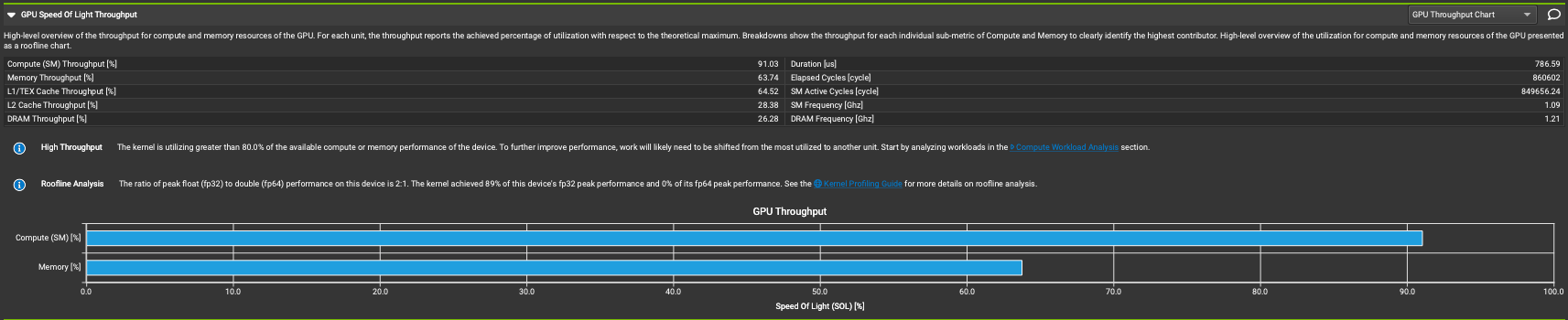
Fig. 19.8 Nsight Compute GUI for Visualizing the SM and Memory throughput of the ampere_gcgemm_64x64_nt kernel.#
In addition to the above GPU throughput, Nsight Compute provides very detailed insight of each kernel and suggests optimization recommendations on other metrics. For example Inspect Memory Workload section builds a visualization of memory transfer sizes and throughput on the profiled architecture, as well as a guide for improving performance.
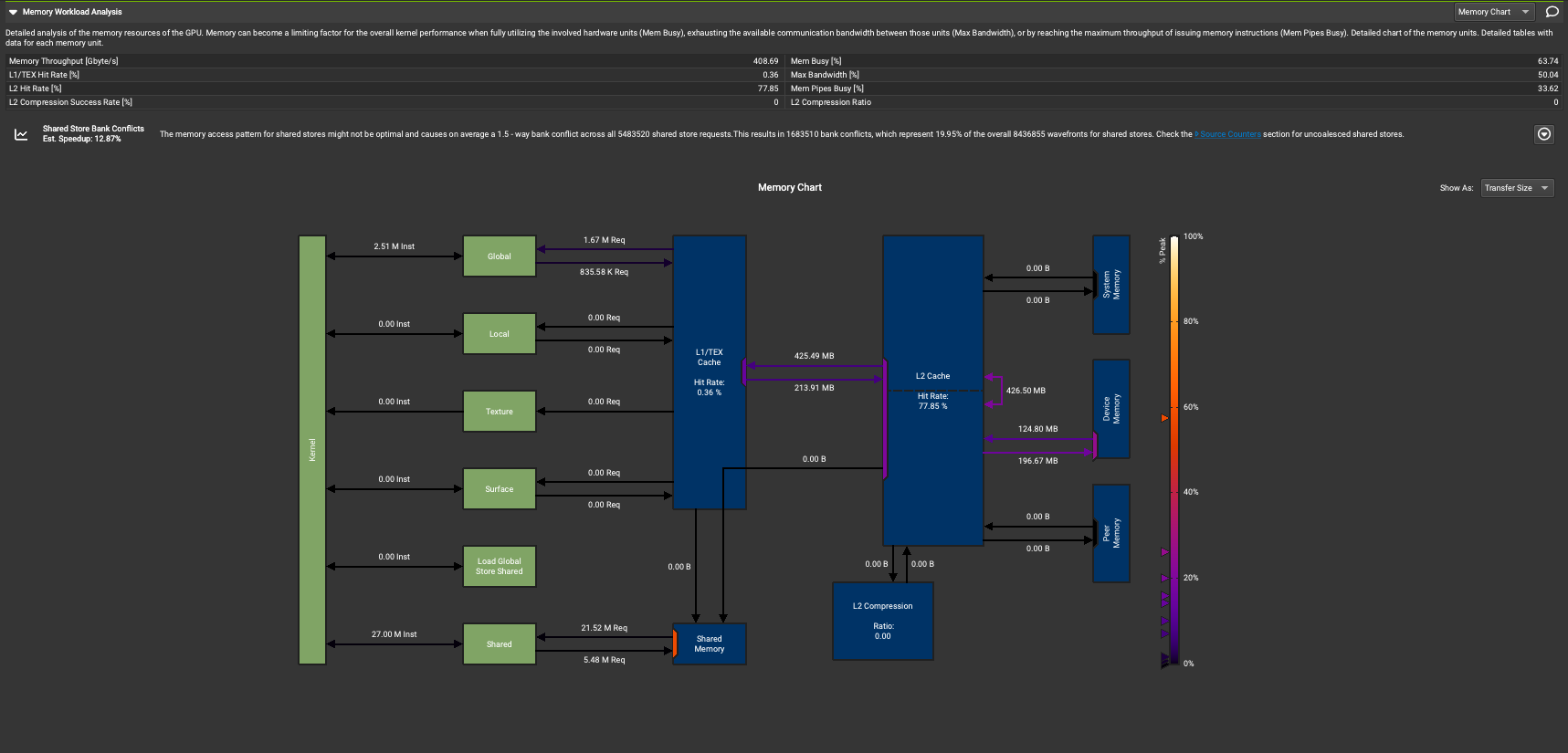
Fig. 19.9 Nsight Compute GUI for Visualizing Transfer Sizes and Throughput on the Memory Hierarchy.#
See also
To see other analysis Nsight Compute provides refer to https://docs.nvidia.com/nsight-compute/ProfilingGuide/index.html#id11
To download the Nsight System and Nsight Compute GUIs on your local machine please follow the instructions here and here respectively.